Bayesian A/B Testing with a Log-Normal Model
In my first blog post I introduced the general framework of Bayesian $$A/B$$ testing, and went into gory details on how to make it happen with binary data: 0, 1, 0, 1, 0, 0, 0…
In the second blog post I went over how to do these kinds of tests on normally distributed data. But what if you have other types of data? Like, say, order values, revenue per session, or time spent on page? Notice that all of these measurements are non-negative or positive, as are many of the metrics we measure & report on at RichRelevance. This means we shouldn’t model the data as being drawn from the battle-tested Gaussian (normal) distribution, because the Gaussian function stretches from negative infinity to positive infinity, and we know for a fact that negative values appear with probability zero. (Although human height, despite being strictly positive, is famously well-modeled by a normal.)
In the realm of strictly positive data (no zeroes!), the log-normal distribution is very common across the sciences and in finance. And, in practice, it fits our data better than other distributions on the same domain (I tried a good portion of these). Here is a histogram of some real order values (excluding zeros), and the log-normal fit:
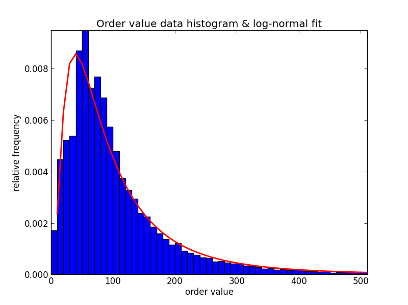
Look at that well-fit tail! Also, notice that a Pareto (power law) distribution is not quite right here because the histogram rises at first and only then tapers off.
So, what next? We now know all about Bernoullis, Binomials, and Gaussians, but log-normals? The easiest way to deal with log-normal data is to remember why the distribution is called log-normal in the first place. Quoth Wikipedia:
If $$X sim operatorname{Log-mathcal{N}}(mu, sigma^2)$$ is distributed log-normally, then $$ln(X) sim mathcal{N}(mu, sigma^2)$$ is a normal random variable.
So contrary to what the name might lead you to conclude, a log-normal distribution is not the log of a normal distribution but rather a distribution whose log is normally distributed.
And another clarification: the mean of a log-normal is not $$mu$$ like you would expect, but it is actually $$e^{mu+sigma^2/2}$$; we will use this fact soon.
Just to make sure we believe that Wikipedia quote, I drew samples from a log-normal distribution in Python, plotted its histogram, and then also plotted the histogram of the log of each of the samples [here is the code]:

As expected, after taking the log of some log-normal samples, the result is normally distributed!
a/b test overview
Keeping that in mind, here is the outline of our approach to A/B testing with log-normal models:
1) Take the log of the data samples.
2) Treat the data as normally distributed, and specify posterior distributions of the parameters $$mu_A$$ and $$sigma_A^2$$ using conjugate priors & a Gaussian likelihood. The details and code are in the previous blog post.
3) Draw random samples of $$mu_A$$ and $$sigma_A^2$$ from the posteriors, and transform each of them back into the domain of the original data. The transformation is chosen depending on what you’re comparing between the $$A$$ side and $$B$$ side. If, for example, the comparison is between means of the log-normal, then the transformation is $$e^{mu_A+sigma_A^2/2}.$$ If the comparison is between modes of the log-normal, then use $$e^{mu_A-sigma_A^2}.$$ You can also compare medians, variances, and even entropies!
4) Repeat steps (1) – (3) for the $$B$$ side, and then compute the probability you’re interested in by numerical integration (just like in the first post).
The math & the code
Let’s take a concrete example: running an $$A/B$$ test on the average value of a purchase order (AOV) of an online retailer. We have $$AOV_A$$ on the $$A$$ side and $$AOV_B$$ on the $$B$$ side, and want to answer the question: “What is the probability that $$AOV_A$$ is larger than $$AOV_B$$ given the data from the experiment?” Or, in math (after log-transforming the data):
$$!p(AOV_A > AOV_B | log(text{data})).$$
How do we answer this question? If we model the order values as being drawn from a log-normal distribution, then the AOV is just the mean of that distribution! And, recalling an earlier point, for a log-normal distribution $$mu$$ is not the mean and $$sigma^2$$ is not the variance! The mean of the log-normal distribution is a function of its $$mu$$ and $$sigma^2$$ parameters; in particular, the mean is
$$!e^{mu+sigma^2/2}.$$
Knowing all that, we can rewrite the probability we’re interested in as:
$$!p(AOV_A > AOV_B | log(text{data})) = p(e^{mu_A+sigma_A^2/2} > e^{mu_A+sigma_B^2/2} | log(text{data})).$$
Where the right hand side is a gnarly-looking integral of the joint posterior (don’t stare it for too long):
$$!iintlimits_{e^{mu_A+sigma_A^2/2}>e^{mu_A+sigma_B^2/2}} p(mu_A,sigma^2_A,mu_B,sigma^2_B|log(text{data})) dmu_A dsigma^2_A dmu_B dsigma^2_B.$$
Despite looking somewhat evil, this integral isn’t that bad! Below the integral signs I have lazily put the “region of interest.” It says: take the integral in the region where $$e^{mu_A+sigma_A^2/2}$$ is larger than $$e^{mu_B+sigma_B^2/2}.$$ I have no idea what that region looks like, and I won’t ever need to because we are going to use sampling to do the integration for us. As a quick reminder, here is how numerical integration of a probability distribution works:
- Draw lots of random samples of $$(mu_A,sigma^2_A,mu_B,sigma^2_B)$$ from $$p(mu_A,sigma^2_A,mu_B,sigma^2_B|log(text{data})).$$
- Count the number of those samples that satisfy the condition $$e^{mu_A+sigma_A^2/2}>e^{mu_A+sigma_B^2/2}.$$
- The probability of interest is just the count from step (2) divided by total number of samples drawn. That’s it!
So now all we have to do is figure out how to draw those samples. As before, independence will be very helpful:
$$!p(mu_A,sigma^2_A,mu_B,sigma^2_B|log(text{data})) = p(mu_A,sigma^2_A|log(text{data})) p(mu_B,sigma^2_B|log(text{data})).$$
Hey look! Since we have already established that $$log(text{data})$$ is distributed according to a normal distribution, that means $$p(mu_A,sigma^2_A|log(text{data}))$$ and $$p(mu_B,sigma^2_B|log(text{data}))$$ are both Gaussian posteriors a la the previous blog post (first and second equations). And we already know how to sample from those! Here is a function that (1) log-transforms the data, (2) gets posterior samples of $$mu$$ and $$sigma^2$$ using the function draw_mus_and_sigmas from the previous blog post, and (3) transforms these parameters back into the log-normal domain:
from numpy import exp, log, mean

def draw_log_normal_means(data,m0,k0,s_sq0,v0,n_samples=10000):
    # log transform the data
    log_data = log(data)
    # get samples from the posterior
    mu_samples, sig_sq_samples = draw_mus_and_sigmas(log_data,m0,k0,s_sq0,v0,n_samples)
    # transform into log-normal means
    log_normal_mean_samples = exp(mu_samples + sig_sq_samples/2)
    return log_normal_mean_samples
And here is some code that runs an $$A/B$$ test on simulated data:
from numpy.random import lognormal

# step 1: define prior parameters for inverse gamma and the normal
m0 = 4. # guess about the log of the mean
k0 = 1. # certainty about m.  compare with number of data samples
s_sq0 = 1. # degrees of freedom of sigma squared parameter
v0 = 1. # scale of sigma_squared parameter

# step 2: get some random data, with slightly different means
A_data = lognormal(mean=4.05, sigma=1.0, size=500)
B_data = lognormal(mean=4.00,  sigma=1.0, size=500)

# step 3: get posterior samples
A_posterior_samples = draw_log_normal_means(A_data,m0,k0,s_sq0,v0)
B_posterior_samples = draw_log_normal_means(B_data,m0,k0,s_sq0,v0)

# step 4: perform numerical integration
prob_A_greater_B = mean(A_posterior_samples > B_posterior_samples)
print prob_A_greater_B

# or you can do more complicated lift calculations
diff = A_posterior_samples - B_posterior_samples
print mean( 100.*diff/B_posterior_samples > 1 )
Putting it all together
We now have models to perform Bayesian $$A/B$$ tests for three types if data: Bernoulli data, normal data, and log-normal data. That covers a great many of the data streams we encounter, and you can even combine them without too much trouble. For example, in computing revenue per session (RPS), most of the samples are zero, and zeroes are not modeled by a log-normal model (its support is strictly positive). To deal with this kind of data, you can simply model zero vs. not-zero with the Bernoulli/Beta model, (separately) model the non-zero values with the log-normal model, and them multiply the posterior samples together. An example combining all the functions from all three blog posts:
from numpy.random import beta as beta_dist
from numpy import mean, concatenate, zeros

# some random log-normal data
A_log_norm_data = lognormal(mean=4.10, sigma=1.0, size=100)
B_log_norm_data = lognormal(mean=4.00, sigma=1.0, size=100)
# appending many many zeros
A_data = concatenate([A_log_norm_data,zeros((10000))])
B_data = concatenate([B_log_norm_data,zeros((10000))])

# modeling zero vs. non-zero
non_zeros_A = sum(A_data > 0)
total_A = len(A_data)
non_zeros_B = sum(B_data > 0)
total_B = len(B_data)
alpha = 1 # uniform prior
beta = 1

n_samples = 10000 # number of samples to draw
A_conv_samps = beta_dist(non_zeros_A+alpha, total_A-non_zeros_A+beta, n_samples)
B_conv_samps = beta_dist(non_zeros_B+alpha, total_B-non_zeros_B+beta, n_samples)

# modeling the non-zeros with a log-normal
A_non_zero_data = A_data[A_data > 0]
B_non_zero_data = B_data[B_data > 0]

m0 = 4.
k0 = 1.
s_sq0 = 1.
v0 = 1.

A_order_samps = draw_log_normal_means(A_non_zero_data,m0,k0,s_sq0,v0)
B_order_samps = draw_log_normal_means(B_non_zero_data,m0,k0,s_sq0,v0)

# combining the two
A_rps_samps = A_conv_samps*A_order_samps
B_rps_samps = B_conv_samps*B_order_samps

# the result
print mean(A_rps_samps > B_rps_samps)
Priors are your friends
One final note: this code works extremely poorly if you only have a few samples of data. For example, set the data to be:
from numpy import array
A_data = array([0,0,0,0,0,0,0,0,0,0,10,20,200,0,0,0,0,0])
B_data = array([0,0,0,0,0,0,0,0,0,0,30,10,100,0,0,0,0,0])
And then run the snippet again. The code will run without errors or warnings, but type max(A_rps_samps) into the console and see what pops out. I see: 2.14e+31! What’s going on? Well, the less data you have, the more uncertainty in both $$mu$$ and $$sigma^2$$. In this case it is $$sigma^2$$ that’s the culprit. Because the log-normal mean samples are $$exp(mu+sigma^2/2),$$ it doesn’t take much change in $$sigma^2$$ for the exponential to blow up. And the inverse Gamma distribution that is the conjugate prior over $$sigma^2$$ can get a bit fat-tailed when you have too few samples (fewer than about 50).
But that doesn’t mean we can’t use this methodology in cases of small sample size. Why? Because we can set the prior parameters as we see fit! If you change v0 from 1 to 25, then the max of A_rps_samps drops down to 109.15, a totally reasonable value given that the maximum of our original data is 200. So, don’t just ignore your prior parameters! As its name suggests, the prior distribution is there so you can encode your prior knowledge into the model. In this example, setting v0 to 25 is equivalent to saying “Hey model, there is less uncertainty in the $$sigma^2$$ parameter than it may seem.”
That’s it for Bayesian $$A/B$$ tests. The next blog post will probably be less statistics-esque and more machine learning-y.